Transmission simulator in FBS#
The method of Transmission Simulator (TS) is primarly used direclty in the modal domain. Nevertheless, the concept of attaching a transmission simulator at the interface can be used also in the frequency domain. In this example a frequency based subtructuring is performed on a complex structure. First a transmission simulator is decoupled from the receiver structure and aftewards a source structure is coupled to the receiver structure. At the interface the VPT is used to obtain collocated interface DoFs.
Note
Download example showing a Transmission Simulator (TS) application: 10_TS.ipynb.
Example Datasests and 3D view#
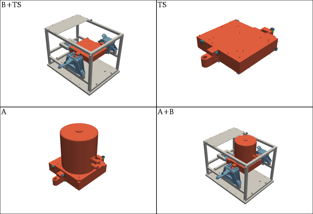
As already shown in the 3D Display one can load the predefined datasets from an example and add a structure from STL file to the 3D display. This allows both the acceleration sensors and excitation points to be visualized. Also for the transmission simulator application, a subplot representation, as already presented in Coupling, can be used.
Virtual point transformation#
The VPT can be performed on experimental data. See the 04_VPT.ipynb example for more options and details.
df_vp = pd.read_excel(xlsx_A, sheet_name='VP Channels')
df_vpref = pd.read_excel(xlsx_A, sheet_name='VP RefChannels')

vpt_TS = pyFBS.VPT(df_chn_TS,df_imp_TS,df_vp,df_vpref,sort_matrix = False)
vpt_BTS = pyFBS.VPT(df_chn_BTS,df_imp_BTS,df_vp,df_vpref,sort_matrix = False)
vpt_A = pyFBS.VPT(df_chn_A,df_imp_A,df_vp,df_vpref,sort_matrix = False)

vpt_TS.apply_VPT(freq,Y_TS)
vpt_BTS.apply_VPT(freq,Y_BTS)
vpt_A.apply_VPT(freq,Y_A)

Y_TS_tran = vpt_TS.vptData
Y_BTS_tran = vpt_BTS.vptData
Y_A_tran = vpt_A.vptData
LM-FBS coupling and decoupling#
First, construct an admittance matrix for the uncoupled system, containing substructure admittances:
Y_AnB = np.zeros((800,30+36+18,30+36+18),dtype = complex)

Y_AnB[:,0:36,0:36] = Y_BTS_tran
Y_AnB[:,36:36+30,36:36+30] = -1*Y_TS_tran
Y_AnB[:,30+36:,30+36:] = Y_A_tran
Next the compatibility and the equilibrium conditions has to be defined through the signed Boolean matrices Bu and Bf.
k = 18
Bu = np.zeros((2*k,36+30+18))
Bu[:k,0:k] = 1*np.eye(k)
Bu[:k,36:36+k] = -1*np.eye(k)

Bu[k:,0:k] = 1*np.eye(k)
Bu[k:,36+30:36+30+k] = -1*np.eye(k)

Bf = np.zeros((2*k,36+30+18))
Bf[:k,0:k] = 1*np.eye(k)
Bf[:k,36:36+k] = -1*np.eye(k)

Bf[k:,0:k] = 1*np.eye(k)
Bf[k:,36+30:36+30+k] = -1*np.eye(k)


Apply the LM-FBS based on the defined coompatibility and equilibrium conditions.
Y_ABn = np.zeros_like(Y_AnB,dtype = complex)

Y_int = Bu @ Y_AnB @ Bf.T
Y_ABn = Y_AnB - Y_AnB @ Bf.T @ np.linalg.pinv(pyFBS.TSVD(Y_int,reduction = 22)) @ Bu @ Y_AnB
First extract the FRFs at the reference DoFs:
arr_out = [30,31,32,33,34,35]
arr_in = [30,31,32,33,34,35]

Y_AB_coupled = Y_ABn[:,arr_out,:][:,:,arr_in]
Y_AB_ref = Y_AB_ref[:,:,:]
Finnaly, the coupled and the reference results can be compared and evaluated:
That’s a wrap!
Want to know more, see a potential application? Contact us at info.pyfbs@gmail.com!