SVT example#
Singular Vector Transformation (SVT) consists in projecting the acquired data into subspaces composed by dominant singular vectors, which are extracted directly from the available FRF datasets. No geometrical and/or analytical model is required. If some basic requirements are met, the reduced orthonormal frequency dependent basis would be able to control and observe most of the rigid and flexible vibration modes of interest over a broad frequency range. The SVT can tackle challenging scenarios with flexible behaving interfaces and lightly damped systems. The method combines reduction with filtering and regularization. It shows an overall low sensitivity to measurement error and significantly reduces the condition number of the interface problem. 1
Note
Download example showing the basic use of the SVT: 18_SVT.ipynb
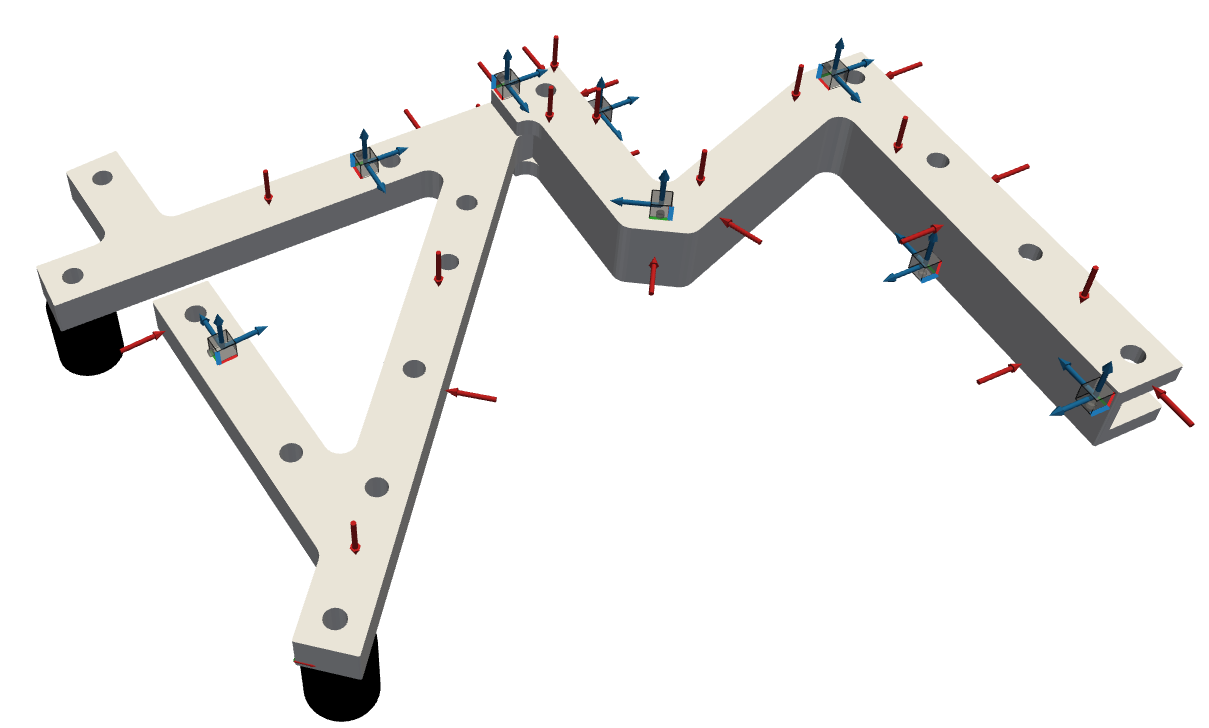
Consider an example for the SVT where 21 impacts and 21 sensor channels are shared between the subsystem B and the B part of system AB within a decoupling application:
Singular Vector Transformation#
The sensor channels (df_chn_B) and impacts (df_imp_B) involved in the transformation process must be assigned. The grouping number (group) is given to simplify the DoFs selection process.
Then, the frequency vector (freq_B) and the FRF matrix (FRF_B) from which the reduced singular subspaces are extracted need to be defined. The integer (n_svs) defines the chosen amount of retained singular component along the frequency range of interest.
As a result, a class instance of pyFBS.SVT can be created.
svt = pyFBS.SVT(df_chn_B,df_imp_B,freq,FRF_B,group,n_svs)
The reduction matrices corresponding to displacement and force transformation from the measured to the singular domain are available as class variables svt.Tu and svt.Tf.
Application of the SVT#
After the reduction matrices are defined, the SVT can be applied directly on the FRF datasets involved in the substructuring scheme.
_,_,FRF_B_sv= svt.apply_SVT(df_chn_B,df_imp_B,freq_B,FRF_B)
_,_,FRF_AB_sv= svt.apply_SVT(df_chn_AB,df_imp_AB,freq_AB,FRF_AB)
Consistency check#
The consistency of the applied transformation can be evaluated by comparing the measured FRFs with the SVT-filtered (reduced and back-transformed) ones.
The filtered FRFs can be obtained by using the class variables svt.Fu and svt.Ff.
FRF_B_filt=np.zeros_like(FRF_B,dtype = complex)
FRF_AB_filt=np.zeros_like(FRF_AB,dtype = complex)
for i in np.arange(len(svt.freq)):
    FRF_B_filt[i,:,:]=svt.Fu[i,:,:] @ FRF_B[i,:,:]@ svt.Ff[i,:,:]
    FRF_AB_filt[i,:,:]=svt.Fu[i,:,:] @ FRF_AB[i,:,:]@ svt.Ff[i,:,:]
That’s a wrap!
Want to know more, see a potential application? Contact us at info.pyfbs@gmail.com!
References
- 1
F.Trainotti, T.Bregar, S.W.B.Klaassen and D.J.Rixen. Experimental Decoupling of Substructures by Singular Vector Transformation. in: Mechanical System and Signal Processing (‘Under Review’), 2021