Virtual Point Transformation#

So… You want to couple two substructures and you already know you need to measure frequency response functions for all translational and rotational degrees of freedom directly at the interface. But you can’t even reach the interface with standard tri-axial accelerometers due to the geometry of the interface? And what about the rotational degrees of freedom?

../../_images/pic_vpt.png — VPT example#

../../_images/seven_three.png — FBS Coupling with VPT#

In general, the main challenges when coupling two substructures can be summarized with the following points:

Non-collocated degrees of freedom on neighboring substructures.
Lack of rotational degrees of freedom due to limitations in measurement equipment and excitation capabilities.
Random and systematic measurement errors.

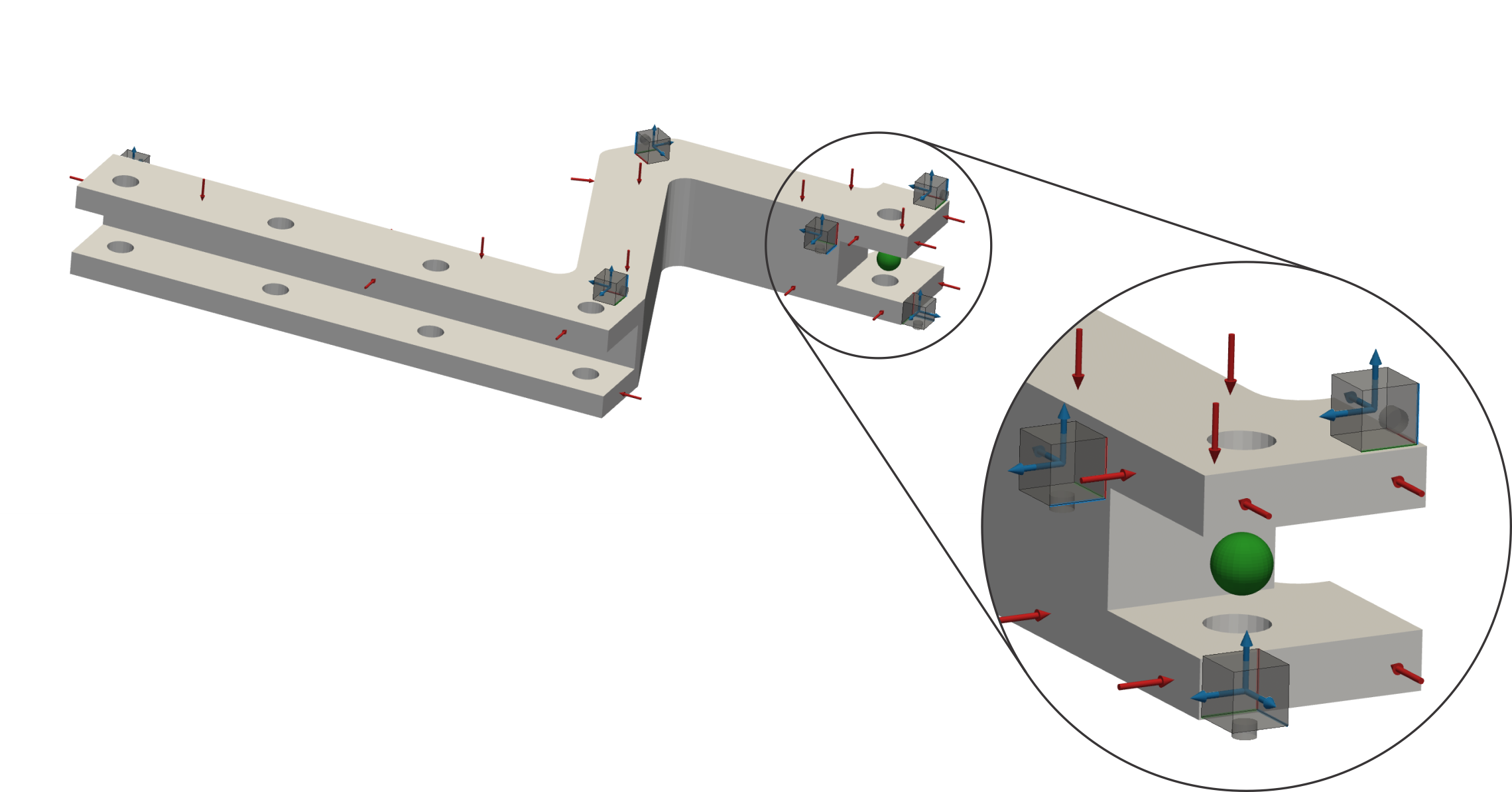
Above-mentioned difficulties can be elegantly overcome using virtual point transformation (VPT). Let us consider a simple interface where the response is captured using tri-axial accelerometers and excited with unidirectional forces around the interface as depicted below. The virtual point is placed in the middle of the hole.

Virtual point displacements#

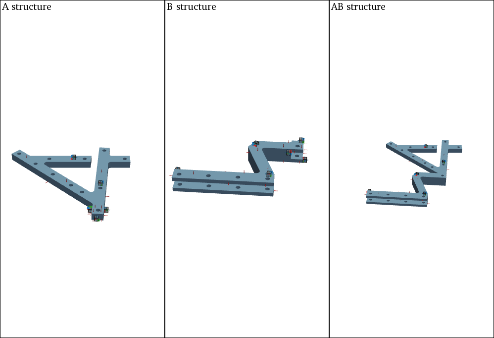
If we observe only the interface, the modes that dominantly represent its response are the translational motions in \(x\), \(y\) and \(z\) axis, as well as rotations about \(x\), \(y\) and \(z\) axis 1. These are named interface deformation modes (IDMs) 2.

In the following, we assume rigid IDMs are dominant while flexible IDMs can be neglected. If we would select one point at the interface (virtual point), an arbitrary channel at \(i\)-th sensor is then rigidly connected to that point.

If we treat interface as perfectly rigid, the VP has six rigid displacements \(\boldsymbol{q}=[q_X,q_Y,q_Z,q_{\theta_X},q_{\theta_Y},q_{\theta_Z}]^\text{T}\). Displacement \(u_x^i\) can be expressed from \(\boldsymbol{q}\); one musk ask himself, which movements of the VP contribute to the \(u_x^i\) response (in the VP coordinate system \(XYZ\)):

\[u_x^i = \underbrace{1 \cdot q_X}_\mathrm{contribution\,from\,\textit{X}\,translation} + 0 \cdot q_Y + 0 \cdot q_Z + 0 \cdot q_{\theta_X} + \underbrace{r_Z \cdot q_{\theta_Y}}_\mathrm{contribution\,from\,\textit{Y}\,rotation} - \underbrace{r_Y \cdot q_{\theta_Z}}_\mathrm{contribution\,from\,\textit{Z}\,rotation}\]

Similarly, responses \(u_y^i\) and \(u_z^i\) are obtained from \(\boldsymbol{q}\) and the relation between one tri-axial sensor and a virtual point can be written as follows:

\[\begin{split}\begin{bmatrix} u_x^i \\ u_y^i \\ u_z ^i \end{bmatrix} = \begin{bmatrix} 1 & 0 & 0 & 0 & r_Z & -r_Y \\ 0 & 1 & 0 & -r_Z & 0 & r_X \\ \underbrace{0}_{\text{translation in }X} & \underbrace{0}_{\text{translation in }Y} & \underbrace{1}_{\text{translation in }Z} & \underbrace{r_Y}_{\text{rotation around }x} & \underbrace{-r_X}_{\text{rotation around }y} & \underbrace{0}_{\text{rotation around }Z} \end{bmatrix} \begin{bmatrix} q_X \\ q_Y \\ q_Z \\ q_{\theta_X} \\ q_{\theta_Y} \\ q_{\theta_Z} \end{bmatrix}\end{split}\]

Columns of the \(\mathbf{R}\) matrix are rigid IDMs, which are assembled from relative sensor position with regard to the VP. For cases where the orientation of sensor channels and VP mismatch, IDMs are transformed in the direction of the sensor channels 2:

\[\begin{split}\begin{bmatrix} u_x^i \\ u_y^i \\ u_z ^i \end{bmatrix} = \begin{bmatrix} e_{x,\,X} & e_{x,\,Y} & e_{x,\,Z} \\ e_{y,\,X} & e_{y,\,Y} & e_{y,\,Z} \\ e_{z,\,X} & e_{z,\,Y} & e_{z,\,Z} \end{bmatrix} \begin{bmatrix} 1 & 0 & 0 & 0 & r_Z & -r_Y \\ 0 & 1 & 0 & -r_Z & 0 & r_X \\ 0 & 0 & 1 & r_Y & -r_X & 0 \end{bmatrix}\, \boldsymbol{q} \quad \Rightarrow \quad \boldsymbol{u}^i = \mathbf{R}_i \, \boldsymbol{q}\end{split}\]

where \([e_{x,X}, e_{x,Y}, e_{x,Z}]^\text{T}\) is orientation of \(x\) sensor channel, \([e_{y,X}, e_{y,Y}, e_{y,Z}]^\text{T}\) is orientation of \(y\) sensor channel and \([e_{z,X}, e_{z,Y}, e_{z,Z}]^\text{T}\) is orientation of \(z\) sensor channel, all in \(XYZ\) coordinate system. Two tri-axial accelerometers are not sufficient to properly describe \(\boldsymbol{q}\) as it is not possible to describe all three rotations with only two tri-axial sensors only. Therefore, it is suggested to use three or more tri-axial accelerometers and the reduction of measurements is performed 2. The use of laser vibrometers 3 or rotational accelerometers in VPT is also encouraged 4 as both yield promising results 5. All relations between measured sensors displacements \(\boldsymbol{u}\) and \(\boldsymbol{q}\) can be assembled into:

\[\begin{split}\begin{bmatrix} \boldsymbol{u}^1 \\ \boldsymbol{u}^2 \\ \boldsymbol{u}^3 \\ \vdots \end{bmatrix} = \begin{bmatrix} \mathbf{R}_1 \\ \mathbf{R}_2 \\ \mathbf{R}_3 \\ \vdots \\ \end{bmatrix} \, \boldsymbol{q} \quad \Rightarrow \quad \boldsymbol{u} = \mathbf{R}\,\boldsymbol{q}\end{split}\]

Since the interface rigidity assumption is not always fully satisfied, a residual term \(\boldsymbol{\mu}\) is added which represents the flexible motion not comprised within rigid IDMs:

\[\boldsymbol{u} = \mathbf{R}\,\boldsymbol{q} + \boldsymbol{\mu}\]

To find the solution \(\boldsymbol{q}\) that best approximates the measured response \(\boldsymbol{u}\), a residual cost function \(\boldsymbol{\mu}^\text{T}\boldsymbol{\mu}\) has to be minimized 6. A solution is found in a least-square sense:

\[\boldsymbol{q} = \Big( \mathbf{R}^{\text{T}} \mathbf{R} \Big)^{-1} \mathbf{R}^{\text{T}} \, \boldsymbol{u} = \mathbf{T}_{\text{u}} \,\boldsymbol{u} \quad \Rightarrow \quad \mathbf{T}_{\text{u}} = \Big( \mathbf{R}^{\text{T}} \mathbf{R} \Big)^{-1} \mathbf{R}^{\text{T}}\]

To gain more flexibility over the transformation, symmetric weighting matrix \(\mathbf{W}\) is introduced 2. If necessary, one could add more weight or even exclude specific displacements from the VPT. The \(\mathbf{W}\) can also be defined per frequency line, so various displamenets can be managed across the entire frequency range.

\[\boldsymbol{q} = \Big( \mathbf{R}^{\text{T}} \mathbf{W} \mathbf{R} \Big)^{-1} \mathbf{R}^{\text{T}} \mathbf{W} \, \boldsymbol{u} = \mathbf{T}_{\text{u}} \, \boldsymbol{u} \quad \Rightarrow \quad \mathbf{T}_{\text{u}} = \Big( \mathbf{R}^{\text{T}} \mathbf{W} \mathbf{R} \Big)^{-1} \mathbf{R}^{\text{T}} \mathbf{W}\]

The matrix \(\mathbf{T}_u\) is a displacement transformation matrix that projects translational displacements into a subspace composed by six rigid IDMs, retaining only the dynamics that load the interface in a purely rigid manner. The residual flexibility is filtered out from \(\boldsymbol{q}\). For cases where the interface exhibits non-neglectable flexible behaviour, additional DoFs can be added to the VP to describe this flexible motion 7.

Virtual point forces#

Similar procedure is applied to transform interaface loads onto the VP. Virtual forces and moments \(\boldsymbol{m}=[m_X,m_Y,m_Z,m_{\theta_X},m_{\theta_Y},m_{\theta_Z}]^\text{T}\) as a consequence of a single unidirectional (\(i\)-th) impact are expressed as (note that forces \(\boldsymbol{f}\) are not uniquely defined by \(\boldsymbol{m}\) as there are infinitely many possible solutions for \(\boldsymbol{f}\)) 2:

\[\begin{split}\begin{bmatrix} m_X \\ m_Y \\ m_Z \\ m_{\theta_X} \\ m_{\theta_Y} \\ m_{\theta_Z} \end{bmatrix} = \begin{bmatrix} 1 & 0 & 0 \\ 0 & 1 & 0 \\ 0 & 0 & 1 \\ 0 & -r_Z & r_Y \\ r_Z & 0 & -r_X \\ -r_Y & r_X & 0 \end{bmatrix}\begin{bmatrix}e_X \\ e_Y \\ e_Z \end{bmatrix}f^i \quad \Rightarrow \quad \boldsymbol{m} = \mathbf{R}_i^\text{T} f^i\end{split}\]

where vector \([e_X,\,e_Y,\,e_Z]^\text{T}\) is the direction of the impact. If we assemble all relations between virtual loads \(\boldsymbol{m}\) and (preferably 9 or more) forces \(f\) we obtain:

\[\begin{split}\boldsymbol{m} = \begin{bmatrix}\mathbf{R}_1 \\ \mathbf{R}_2 \\ \mathbf{R}_3 \\ \vdots\end{bmatrix} \boldsymbol{f} \quad \Rightarrow \quad \boldsymbol{m} = \mathbf{R}^\text{T} \boldsymbol{f}\end{split}\]

The problem now is underdetermined and forces \(\boldsymbol{f}\) are found by standard optimization. Optimal solution is the one that minimizes cost function \(\boldsymbol{f}^\text{T}\boldsymbol{f}\) while subjected to \(\mathbf{R}^\text{T} \boldsymbol{f} - \boldsymbol{m} = \mathbf{0}\) 6:

\[\boldsymbol{f} = \mathbf{R}\left(\mathbf{R}^\text{T} \mathbf{R} \right)^{-1} \boldsymbol{m} = \mathbf{T}^\text{T}_\text{f} \,\boldsymbol{m} \quad \Rightarrow \quad \mathbf{T}^\text{T}_\text{f} = \mathbf{R}\left(\mathbf{R}^\text{T} \mathbf{R} \right)^{-1}\]

Preferences in measurement data may be given using weightening matrix:

\[\boldsymbol{f} = \mathbf{W}\mathbf{R}\left(\mathbf{R}^\text{T} \mathbf{W} \mathbf{R} \right)^{-1} \boldsymbol{m} = \mathbf{T}^\text{T}_\text{f}\, \boldsymbol{m} \quad \Rightarrow \quad \mathbf{T}^\text{T}_\text{f} = \mathbf{W}\mathbf{R}\left(\mathbf{R}^\text{T} \mathbf{W} \mathbf{R} \right)^{-1}\]

Virtual point admittance#

With both transformation matrices, virtual point FRFs can be computed using 2:

\[\mathbf{Y}_{\text{qm}} = \mathbf{T}_{\text{u}} \, \mathbf{Y}_{\text{uf}} \, \mathbf{T}^{\text{T}}_{\text{f}}\]

where \(\mathbf{Y}_{\text{uf}}\) is the measured FRF matrix and \(\mathbf{Y}_{\text{qm}}\) is the full-DoF VP FRF matrix with perfectly collocated motions and loads. That means that the VP FRF matrix should be reciprocal.

For the driving-point FRFs at the diagonal of the matrix, passivity can be evaluated since the driving-point FRF should always be minimum-phase function:

\[\begin{split}\angle \mathbf{Y}_{ii} = \begin{cases} \in [-180^{\circ},\,0^{\circ}] \quad &\text{for receptance FRFs}\\ \in [-90^{\circ},\,90^{\circ}] \quad &\text{for mobility FRFs}\\ \in [0^{\circ},\,180^{\circ}] \quad &\text{for accelerance FRFs} \end{cases}\end{split}\]

Measurement quality indicators#

Measurement quality indicators compare original responses with responses transformed into VP and then projected back to the initial location 8. A good agreement between responses indicates, that the transformation is performed correctly in a physical sense. If vector \(\boldsymbol{q}\) is known, expansion of responses to the \(\boldsymbol{u}\) is also possible. However, as there is no flexible motion in \(\boldsymbol{q}\), there is also no flexible motion in reconstructed \(\boldsymbol{u}\) for that is filtered out. Therefore, we introduce \(\boldsymbol{\tilde{u}}\), reconstructed filtered displacements:

\[\tilde{\boldsymbol{u}} = \mathbf{R}\, \boldsymbol{q} = \mathbf{R} \Big( \mathbf{R}^{\text{T}} \mathbf{W} \mathbf{R} \Big)^{-1} \mathbf{R}^{\text{T}} \mathbf{W}\, \boldsymbol{u} = \mathbf{F}_{\text{u}}\,\boldsymbol{u}\quad \Rightarrow \quad \mathbf{F}_{\text{u}} = \mathbf{R}\,\mathbf{T}_{\text{u}} = \mathbf{R}\,\Big( \mathbf{R}^{\text{T}} \mathbf{W} \mathbf{R} \Big)^{-1} \mathbf{R}^{\text{T}} \mathbf{W}\]

\[\boldsymbol{u} = \mathbf{Y} \boldsymbol{f}\]

\[\tilde{\boldsymbol{u}} = \mathbf{F}_\text{u} \mathbf{Y} \boldsymbol{f}\]

Overall sensor consistency is calculated from norms of filtered and non-filtered responses:

\[\boldsymbol{\rho}_\boldsymbol{u} = \frac{||\tilde{\boldsymbol{u}}||}{||\boldsymbol{u}||}\]

Values of \(\rho_\boldsymbol{u}\) close to 1 indicate that all sensors are correctly positioned, aligned, and calibrated. Low values at higher frequencies indicate the presence of flexible interface modes. Specific sensor consistency is evaluated per measurement channel with the use of coherence criterion:

\[\rho_{{u}_i} = \text{coh}(\tilde{u}_i,\,u_i) \quad \tilde{u}_i\,\in\,\tilde{\boldsymbol{u}},\,u_i\,\in\,\boldsymbol{u}\]

Using specific sensor consistency a sensor with incorrect position, direction or calibration can be identified. A similar procedure is also used to evaluate the overall and specific quality of individual impacts. Sum of responses for each impact is defined:

\[\boldsymbol{y} = \boldsymbol{w}^\text{T}\mathbf{Y}\]

Sum of responses is calculated again, but this time for forces first projected onto the VP and then back-projected to the initial location:

\[\tilde{\boldsymbol{y}} = \boldsymbol{w}^\text{T}\mathbf{Y}\mathbf{F}_\text{f} \quad \Rightarrow \quad \mathbf{F}_\text{f} = \mathbf{R} \mathbf{T}_\text{f}\]

Overall impact consistency is calculated as follows:

\[\boldsymbol{\rho}_\boldsymbol{f} = \frac{||\tilde{\boldsymbol{y}}^\text{T}||}{||\boldsymbol{y}^\text{T}||}\]

A high value of the overall impact consistency indicator implies that the impact forces can be fully represented by the rigid IDMs. Specific impact consistency is evaluated as:

\[\rho_{{f}_i} = \text{coh}(\tilde{y}_i,\,y_i) \quad \tilde{y}_i\,\in\,\tilde{\boldsymbol{y}},\,y_i\,\in\,\boldsymbol{y}\]

A low specifc impact consistency values can indicate an incorrect position, direction, double impact or that the impact resulted in signal overload at any channel.

References

1: de Klerk D, Rixen DJ, Voormeeren SN, Pasteuning P. Solving the RDoF problem in experimental dynamic sybstructuring. InInternational modal analysis conference IMAC-XXVI 2008 (pp. 1-9).
2(1,2,3,4,5,6): van der Seijs MV, van den Bosch DD, Rixen DJ, de Klerk D. An improved methodology for the virtual point transformation of measured frequency response functions in dynamic substructuring. In4th ECCOMAS thematic conference on computational methods in structural dynamics and earthquake engineering 2013 Jun (No. 4).
3: Trainotti, Francesco, Tobias FC Berninger, and Daniel J. Rixen. Using Laser Vibrometry for Precise FRF Measurements in Experimental Substructuring. Dynamic Substructures, Volume 4. Springer, Cham, 2020. 1-11.
4: Tomaž Bregar, Nikola Holeček, Gregor Čepon, Daniel J. Rixen, and Miha Boltežar. Including directly measured rotations in the virtual point transformation. Mechanical Systems and Signal Processing, 141:106440, July 2020.
5: Bregar T, El Mahmoudi A, Čepon G, Rixen DJ, Boltežar M. Performance of the Expanded Virtual Point Transformation on a Complex Test Structure. Experimental Techniques. 2021 Feb;45(1):83-93.
6(1,2): Häußler, Michael, and Daniel Jean Rixen. Optimal transformation of frequency response functions on interface deformation modes. Dynamics of Coupled Structures, Volume 4. Springer, Cham, 2017. 225-237.
7: Pasma EA, van der Seijs MV, Klaassen SW, van der Kooij MW. Frequency based substructuring with the virtual point transformation, flexible interface modes and a transmission simulator. InDynamics of Coupled Structures, Volume 4 2018 (pp. 205-213). Springer, Cham.
8: van der Seijs MV. Experimental dynamic substructuring: Analysis and design strategies for vehicle development (Doctoral dissertation, Delft University of Technology).

Frequency Based Substructuring

VPT example