Singular Vector Transformation#
Singular Vector Transformation (SVT) consists in projecting the acquired data into subspaces composed by dominant singular vectors, which are extracted directly from the available FRF datasets. No geometrical and/or analytical model is required. If some basic requirements are met, the reduced orthonormal frequency dependent basis would be able to control and observe most of the rigid and flexible vibration modes of interest over a broad frequency range. The SVT can tackle challenging scenarios with flexible behaving interfaces and lightly damped systems.
SVT example#
FBS Decoupling with SVT#
Singular value decomposition#
The singular value decomposition can be used to decompose and sort the dynamical information of the measured FRF dataset:
where \(\mathbf{U}(\omega)\) and \(\mathbf{V}(\omega)\) are the orthonormal frequency-dependent left and right singular vectors and \(\mathbf{\Sigma}(\omega)\) is the diagonal matrix containing the non-negative singular values of the matrix.
The column vectors of \(\mathbf{U}(\omega)\) and \(\mathbf{V}(\omega)\) can be considered as approximate mode shapes and approximate modal participation factors at the frequency \(\omega\). The associated singular values are the scaling factors representing how dominant the contribution (dynamically) of a singular state is at that frequency.
Note
Note how the singular ‘motions’ are frequency dependent and span an orthogonal space (mathematical orthogonality), while the characteristic modal vectors are frequency independent and are \(\mathbf{K}\)-orthogonal and \(\mathbf{M}\)-orthogonal (physical orthogonality).
Tip
Idea! Why don’t we use the singular vectors as reduction bases to weaken the interface problem?
A subset of dominant singular vectors in \(\mathbf{U}(\omega)\) and \(\mathbf{V}(\omega)\) could be used to construct meaningful reduction spaces that naturally contain rigid as well as flexible local interface deformations.
Methodology#
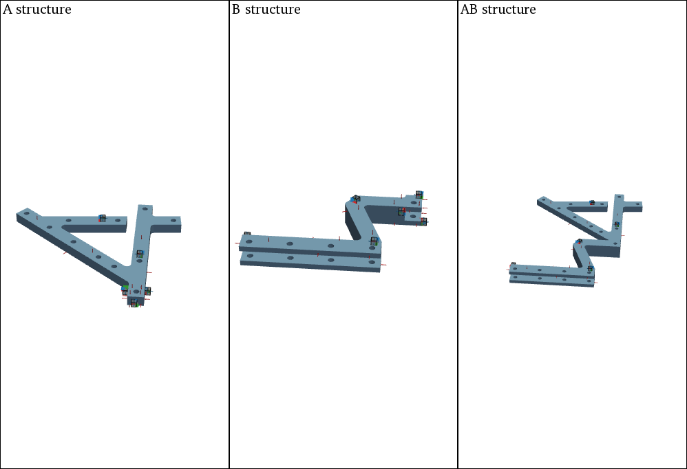
An extended (direct) decoupling problem is considered, where the goal is finding the interface forces that suppress the influence of A on AB, thus isolating the uncoupled response of subsystem B.

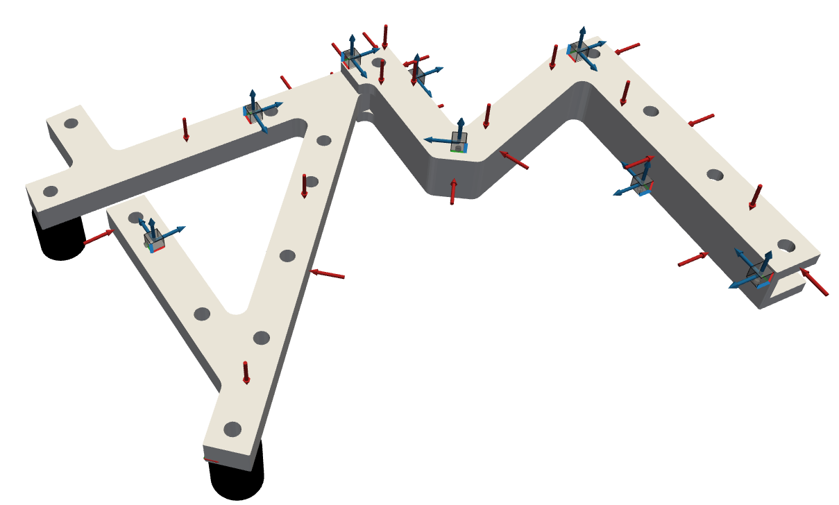
Let’s assume collocation between the inputs between AB and A and outputs between AB and A. Let’s also assume that inputs and outputs do not share the same location and are distributed all over the common area between AB and A (interface and internal) such that the interface deformation of interest is controlled and observed in a similar manner.
The proposed procedure is summarized 1:
Place inputs and outputs in a collocated manner between AB and A. Distribute them homogeneously over the full area (interface and internal), such that all the vibration modes of interest are controlled and observed through similar dynamic spaces.
Perform a SVD on \(\mathbf{Y}^\text{A}\), such that \(\mathbf{Y}^\text{A}=\mathbf{U}^\text{A}\mathbf{\Sigma}^\text{A}(\mathbf{V}^\text{A})^\text{H}\).
Select truncated basis of left- and right SVs \(\mathbf{U}_r^\text{A}\), \(\mathbf{V}_r^\text{A}\) for the reduction of measured displacements and forces. The subspaces’ vectors are complex, orthonormal and frequency-dependent.
Use the same reduction bases for \(\mathbf{Y}^\text{A}\) and \(\mathbf{Y}^\text{AB}\). This is necessary for imposing collocated compatibility and equilibrium between the substructures.
Decouple the reduced components according to the LM-FBS algorithm.
Note
The SVD can be applied analogously on \(\mathbf{Y}^\text{AB}\). For simplicity, the derivation will be performed with the singular bases of \(\mathbf{Y}^\text{A}\).
Mathematical derivation#
Let’s apply an SVD on the measured dataset \(\mathbf{Y}^\text{A}\):
The left and right singular subspaces are complex orthonormal frequency-dependent bases. Proper reduced bases \(\mathbf{U}_r^\text{A}\) and \(\mathbf{V}_r^\text{A}\) are chosen per frequency line according to a user-defined criteria. The frequency dependence will be omitted for simplicity from here on.
Displacement reduction#
The same reduction basis \(\mathbf{U}_r^\text{A}\) is chosen for A and AB to preserve a collocated compatibility in the reduced domain:
The residual \(\boldsymbol{\mu}^\text{A}\) represent the low-value singular states not included in \(\mathbf{U}_r^\text{A}\). The residual \(\boldsymbol{\mu}^\text{AB}\) indicates the motion of AB that could not be described by the reduced singular subspace of A. The transformation from the measured to the reduced space is obtained as:
where
The superscripts \((\star)^+\) and \((\star)^\text{H}\) denote the Moore-Penrose pseudo-inverse and Hermitian operators respectively.
Note
Note that, due to the orthogonality of \(\mathbf{U}_r\), no mathematical inversion has to be computed.
To check the quality of the transformation, the filtered and measured displacements can be compared:
Force reduction#
The same reduction basis \(\mathbf{V}_r^\text{A}\) is chosen for A and AB to preserve a collocated equilibrium in the reduced domain:
The transformation from the reduced to the measured space is obtained as:
The superscripts \((\star)^+\) and \((\star)^\text{H}\) denote the Moore-Penrose pseudo-inverse and Hermitian operators respectively. The filtered forces can be compared to the measured ones:
Finally, the compatibility and equilibrium conditions are imposed in the reduced space observed by \(\mathbf{U}_r\) and controlled by \(\mathbf{V}_r\) respectively:
Thus, a weakening of the interface problem is obtained. The solution of the equations follows the LM-FBS formulation:
where the reduced uncoupled admittance \(\mathbf{Y}^\text{AB|A}_{\zeta\eta}\) can be written as:
Filtering \(\mathbf{Y}^\text{AB}\) by reduction and back-projection (see filter matrices \(\mathbf{F}_\text{u}\) and \(\mathbf{F}_\text{f}\)) using the singular subspaces of \(\mathbf{Y}^\text{A}\) can be useful to determine how well the local dynamics of AB is described through the reduced dominant controllability and observability spaces of A.
Requirements#
Let’s remind ourselves of the main assumptions for a successful SVT:
Inputs in A and in the A part of AB must be collocated and so must the output in A and in the A part of AB. This is necessary to since no geometrical reduction is applied afterwards. In experimental practice, this requirement should not be too challenging,
Inputs and output spaces should contain the same dynamical information. The balance between controllability and observability spaces is needed to minimize the physical inconsistency of the reduced model. In experimental practice, an homogeneous distribution of inputs and outputs throughout the available common area (A and the A part of AB) should be ensured,
The reduced orthonormal subspaces of A should be able to map the observed and controlled dynamics in AB.
Benefits#
The SVT relies on a simple concept: the measured dynamics is projected into a subspace composed by dominant singular states extracted from the measurement itself. What are the main advantages and features of the SVT?
No need for geometrical/analytical information,
Flexible behaviour potentially included (if properly observed/controlled),
Frequency-dependent transformation,
Efficient least square smoothing of random error and outliers,
Better conditioning of the interface problem,
Reduce sensitivity to measurement location/direction bias.
References
- 1
F.Trainotti, T.Bregar, S.W.B.Klaassen and D.J.Rixen. Experimental Decoupling of Substructures by Singular Vector Transformation. in: Mechanical System and Signal Processing (‘Under Review’), 2021